Introducing the Reflectron
Update 2: Introducing the Reflectron
When a physical wave reaches an interface, it does something interesting: it splits in two. One portion is transmitted through the interface, and the other portion is reflected back into the system. Is this significant in the behavior of real neurons? What if I added this effect into our computational neurons?
I was sidetracked from my studies by this idea which demanded I implement it.
Reflecting on how computational neurons are a rough analogy for biological neurons, I realized many of the details are lost in the modeling process: the complex chemical signaling that innervates the dendrites, is integrated in the soma, and–if above a certain threshold potential (i.e. tanh)–is transmitted down the neuron to the axon terminal, which impacts the complex chemical interplay between neurons. These are actual electric waves flowing through a series of interfaces–like an input signal flowing through our MLP’s DAG. Imagining the potential flowing through networks of neurons reminded me of some past physics work modeling electric waves.
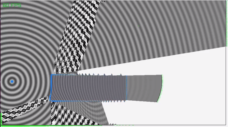
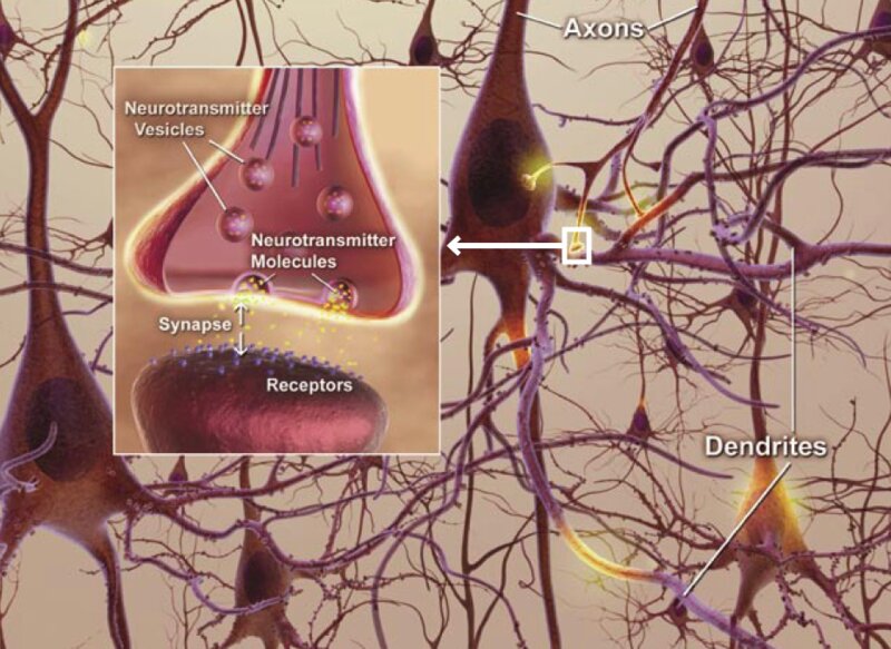
This stood out to me as something that would have a small physical effect with a significant impact on the performance of the biologic neuron, but is one of the many details lost in its digital counterpart. It is easy to imagine that real neurons experience this behavior throughout their structure and between the axons and dendrites–and that the infinite recursion of a physical system enables orders of magnitude more interactions than the simplified model used for neural nets. I wondered if modeling this “reflection” behavior would improve the performance of a neural network.
I figured it would be interesting to see if I could develop a model for a digital neuron that incorporated some of this behavior, and to see how an MLP built from these “internally reflecting neurons”–or Reflectrons–behaved. I hoped the increased computational complexity of each Reflectron would produce greater “information gain” compared to the basic Neuron.
Modeling The New Behavior
When an electric wavefront hits an interface, some portion of the wave is transmitted onward, and some portion is reflected back. Physically, energy is conserved: the “wave” is split into two portions. This repeats at every interface, in both directions–a reflection can reach a previous interface and reflect again to move in the original direction; some portion can also be transmitted backwards to an earlier stage.
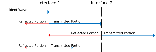
Interface Reflections
Physically this repeats infinitely, though the effect arguably becomes noise after one or two reflections. This is an analogue, time-variant effect with high-order interactions that occurs in a system with time-varying inputs and outputs (e.g. a pulse). That math is vastly different from the neurons I built before, which are completely independent of time and implemented as a Directed Acyclic Graph with micro-gradient backpropagation–neither of which is (to my knowledge) conducive to recursive/cyclic behaviors. These are two very different ways of thinking. The physics perspective thinks about a signal–as an entity itself–moving through a series of stages like a person running through an obstacle course. The math/cs perspective focuses on the stages themselves: the system is a series of operations, each transforming an input into an output, like converting ingredients into a finished meal.
This is the first major challenge I ran into: how do I translate the physical behavior into the mathematical perspective, given the constraints of our computational model? How do I model signal reflections in software built upon the Directed Acyclic Graph?
Puzzling this out took some time, but I found it fun to actually think about these models and what they represent. My solution came in two parts. The first is to introduce a pair of nodes to represent an interface: a Transmission node inserted into the graph, and an associated Reflection node branching off the same edge. The second part is to copy the neuron graph into an additional layer for each reflection, take the reflection node’s value and feed it into an earlier node in the new layer.
The Transmission/Reflection (T/R) nodes share a single alpha parameter, which determines how much of the signal is transmitted or reflected–as one goes up, the other goes down. This became its own Value node in the graph, and was treated like a weight–modified during backpropagation to optimize performance of the network. I also had to introduce a Mixing node to combine (or “mix”) reflected signals into the existing edges of the graph. Both of these created new design choices: how do I model signal transmission/reflection using a single alpha value? Should the mixing be additive or multiplicative? How do I combine the reflections together into a single output Value?
In a physical system, the incident energy is divided between the transmitted or reflected waves–so I initially used a single value multiplied by the output float value to determine the “value transmitted” by that node in the DAG. For reflections, I used for the coefficient. This mostly worked, but broke down as the transmission coefficient was adjusted below zero or above 1. Setting bounds for the values felt like an arbitrary limit to the intended behavior of the graph; so instead I pivoted to using sigmoid function as a rough analogue for the behavior I wanted: and were defined as derivable from another variable , which became the trainable coefficient ( & ). This formulation loses the physical reality of energy conservation, but maintains the general idea of the energy being “split” in a way that aligns with the algorithms at play. It reminds me of some other practices, like adopting Negative Log Likelihood
With respect to mixing: I implemented both, but used additive mixing for most of my testing. It seemed the most direct representation since I was thinking of the Values as “signal energy”. That said, signal amplitudes generally mix multiplicatively, so that may be an area for future experimentation.
So I defined two new nodes: Mixing nodes and Transmission/Reflection nodes. Where do I add them in the Neuron’s graph to model “reflections as new layers”?
Reflectron
I imagined three versions of my new “Reflectron”: one which modeled reflections at the signal level, one which modeled the reflections at the neuron level, and one which modeled reflections at the layer/network level, though the latter is beyond the scope of my effort and may be functionally similar to recursive networks and cyclic graphs, which I haven’t studied yet.
S2S
I started with the Signal-to-Signal (S2S) Reflectron, since it was the most complicated and–I hoped–the most performant. This model required I add a reflection node at each major interface: the reflection would “travel back” to the previous interface, where it could be reflected again to propagate forward. I modeled the reflection as an intermediary layer between the DAG reflection layers: the simple “half-layer” would only add T/R nodes for the initial interface of the previous layer. A “full-layer” would add an additional set of T/R nodes for each signal reflection, to represent the signal reaching the preceding interface. Higher order reflections could be modeled by adding additional layers.
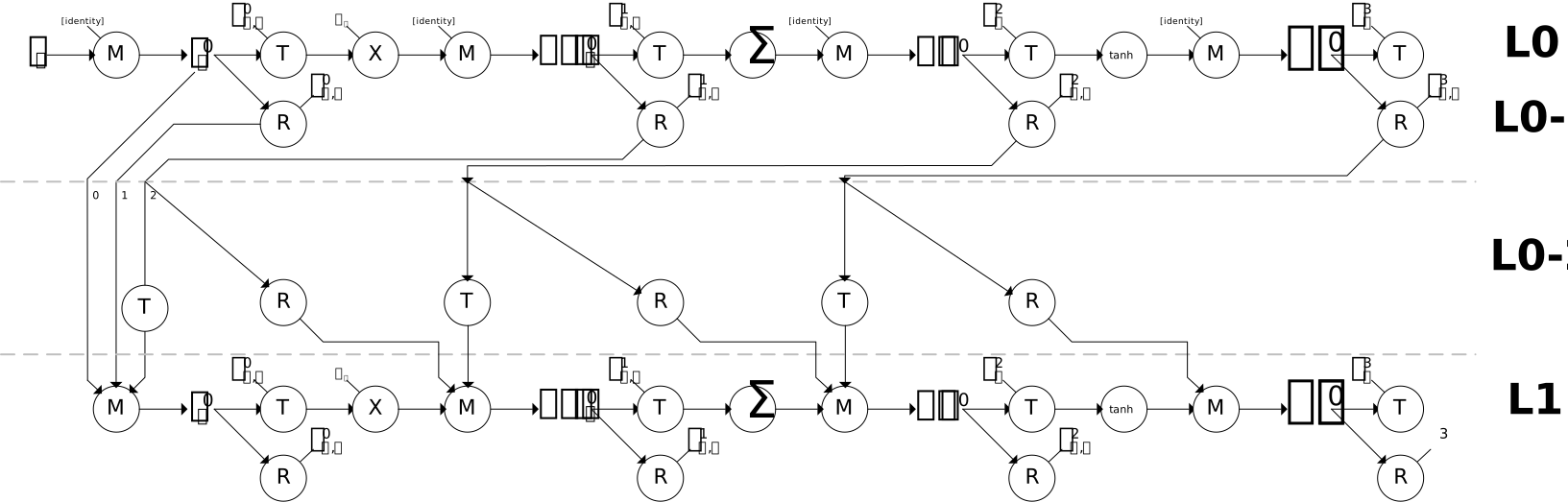
S2S Reflectron Diagram
One aside about memory: I used one of the techniques I learned last time to manage all the T/R alpha variables across the Reflectron’s layers: arena allocation. This allowed me to create a custom 3D+2D hybrid layout that very closely matched the requirements of the Reflectron’s multi-stage DAG (1).
Reflectrons have more tunable parameters compared to the basic neurons I’ve been working with. In order to make the comparison fair, I ran all my tests against both: a) MLPs that used the same number of neurons as reflectrons, and b) MLPs that used additional neurons to have the same “tunable parameter count” as the reflectron version. I ran regression tests across four datasets (iris, circles-3ring, wine, breast cancer) using 10 seeds and 200 epochs (2):
| dataset | MLP eq-neurons | MLP eq-params | SS | Δ vs eq-params | SS params | SS runtime |
|---|---|---|---|---|---|---|
| iris | 0.650 | 0.710 | 0.907 | +0.197 | 163 | ~570 ms |
| circles | 0.990 | 0.983 | 0.733 | −0.250 | 627 | ~2.4 s |
| wine | 0.978 | 0.969 | 0.953 | −0.016 | 1155 | ~5.2 s |
| breast | 0.966 | 0.963 | 0.967 | +0.004 | 1962 | ~27 s |
Note: the iris tests performed better with 50+ seeds, climbing to ~0.95
Full per-seed results for every arm: Data & Tables.
The S2S Reflectron produced results that were–generously–almost as good as the traditional MLP. They didn’t warrant serious development, especially compared to normal neurons with the same parameter count. In most of my testing they cost 2-3x the MLP’s parameters and 5-20x the runtime!
Thinking about it, this makes sense: I haven’t done anything to increase the “density” of the neuron’s behavior. Recently I’ve been wondering how to analyze what a neuron actually does. This led me to thinking about signals in a neural network as having the attribute of Information Density (3), which represents the “amount of meaning” in that signal (separate from a feature’s actual value, which gets multiplied by the weights). A neuron acts to concentrate this meaning, this information, from a set of low density signals into a set of slightly higher density signals. The final output of a neural network would have a very high information density.
I can use this framework to think about why the S2S Reflectron didn’t experience many performance improvements: I’m essentially feeding the signals forward through an identical neuron. Since I chose to perform the mixing at the input of the neuron–so the “main” neuron is actually the bottom layer, which mixes in reflected signals from the layers above it–there isn’t any change in the neuron’s architecture to extract more meaning from the input features compared to just adding more neurons to the network.
With these things in mind, I had three guiding stars to inform my next attempt:
- Excessively expanding the neuron’s graph adds complication without adding performance. This was also evident when adding 3+ reflections did not change test results–so all N2S numbers reported below use num_reflections=1, a single-reflection two-stage graph. Deeper reflection stacks didn’t produce statistically distinguishable gains in my early testing, so the extra parameters and runtime didn’t seem worth it.
- Reflections should modulate the inputs to the neuron. The computed output should “reflect” and modify the inputs.
- Internal neuron modulation does not produce a network DAG that is substantially different from adding more neurons; inter-neuron modulation is necessary.
These changes informed the architectural decision for the next variant, the N2S Reflectron.
N2S
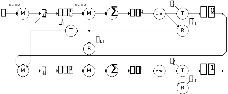
The second, improved version of the Reflectron I implemented is the Neuron-to-Signal variant. This is much simpler, with only two Transmission/Reflection node pairs per layer as opposed to the S2S’s cascade: one pair splitting the post-tanh output and another taking that output’s reflection and splitting it into the beginning or middle of the next stage. This only required two independent leaves per stage (with four derived alphas) instead of the S2S version’s massive array.
N2S Reflectron
The new Reflectron used a much simplified version of the S2S graph. I still used layers to represent reflections as a DAG, but I only insert a single T/R node into the chain–which loops back into the beginning of the neuron’s graph. I also focused on mixing together all the layers at the output nodes, instead of passing the feature value into each layer. This way each layer computes the response to reflection stimulus itself. The result was a Reflectron with solid performance, but minimal gains over regular neurons.
One implementation detail took me a while to find: choosing to mix the outputs (LAYER_MIX_OUTPUTS) was actually my second attempt. I initially used LAYER_MIX_INPUTS, where features cascade through every stage’s first Mixing node and the final stage’s output becomes r->out. That version produced suspiciously flat predictions on every seed. The composed tanh nonlinearities across stages were saturating from the first forward pass, and downstream stages were being fed values outside their own linear regime. Fixing this required Xavier-like weight initialization , which was small enough to keep pre-tanh sums near one. This was a numerical decision that determined if my architecture worked or not; once I implemented the fix both layer-mixing modes worked.
| dataset | MLP eq-neurons | MLP eq-params | N2S | Δ vs eq-params | N2S params | N2S runtime |
|---|---|---|---|---|---|---|
| iris | 0.650 | 0.710 | 0.930 | +0.220 | 91 | ~340 ms |
| circles | 0.990 | 0.983 | 0.987 | +0.004 | 283 | ~1.3 s |
| wine | 0.978 | 0.969 | 0.992 | +0.023 | 459 | ~2.4 s |
| breast | 0.966 | 0.963 | 0.975 | +0.012 | 722 | ~11.8 s |
Full per-seed results for every arm: Data & Tables.
The N2S Reflectron wins or ties every dataset (against equal-parameter MLPs) at 1.1-1.4x the MLP’s parameters and 3-5x the runtime. Notably, MLPs at equal parameter counts to N2S were slightly worse on wine and breast–the extra capacity without additional data can actually hurt the final performance. N2S wins aren’t just “more parameters help”.
The main difference I added was inter-neuron modulation of the features themselves. This was what I originally envisioned: the neuron itself acting as a T/R interface. The “energy” from the input features gets mixed together, and based on the output value of the neuron, some of that energy is bounced back into the input value itself–which changes the inputs of all the other neurons.
I implemented this by taking the reflected value that would be mixed into the beginning of the Reflectron’s next layer and mixing it into the next layer of all the neurons, for that feature.
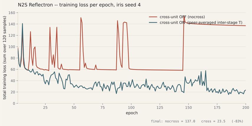
Claiming this wins is still a pretty generous interpretation. These are negligible gains. But there was one interesting result on seed four of the Iris test set: the N2S network collapsed into a degenerate solution, with training accuracy 33.3%, test accuracy 33.3%, and a final loss of 137. Iris is a three-class, balanced dataset; this meant the model learned to predict a single class for every input–resulting in a 5-9x worse performance (loss of 137 vs. a successful iris model’s 15-25). The Reflectron’s tanh non-linearities had reached the saturation region, causing the softmax output to collapse. I think I ran into a case where the gradients stopped being meaningful, trapping the network at a kind of “local minimum”. However, using the same seed/starting weights but enabling cross-unit modulation, the same network achieves a 96.7% train, 100% test, and a loss of 23.5.
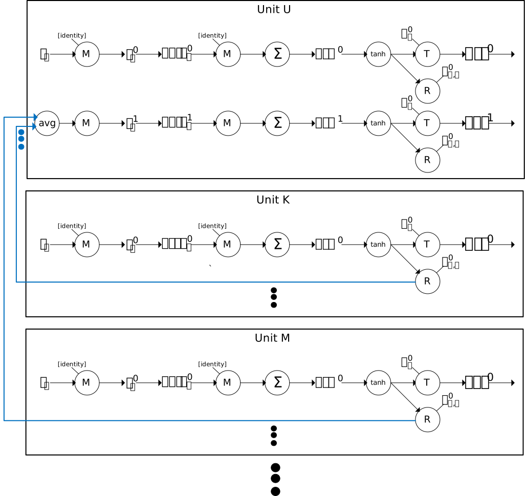
Cross-unit modulation is my first attempt at modeling “cross-talk” between nearby neurons. I imagined that the electrical activity of one neuron would produce a field (or secondary effects in the environment), which would then up-regulate or down-regulate neurons in the vicinity.
- Cross-Unit Modulation Disabled: each unit’s next stage reads only its own reflected signal from the previous one.
- Cross-Unit Modulation Enabled: For each unit U in the layer: take the reflected outputs of all other units in the layer, average them to prevent downstream tanh saturation, and feed that peer-averaged signal into U’s next stage input. This couples units at each inter-stage boundary. It’s superficially similar to attention–mixing contributions from multiple units into one target unit–but using static weights baked into the DAG at construction rather than learned dynamic ones. Replacing the constant averaging with learned softmax-normalized dynamic weights might be an interesting experiment.
Cross-Unit Modulation in a Layer
Even when one unit’s tanh node reaches saturation, the other units still provide a gradient pathway that isn’t routed through the broken non-linearity, thereby acting as a stability rail. The N2S UNIQUE experiment I ran later produced the same rescue on seed four through a different mechanism (per-feature reflection amplitude).
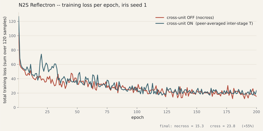
Cross-unit modulation changed every one of iris’s 91 parameters. For example: on iris seed 1 the nocross vs. cross weight configurations are farther apart than either is from the origin (4), yet both reach ~99% test accuracy–effectively the same decision boundary using different paths. The training loss curves visibly diverge from early in the training.
As an aside: iris regularly hit a failure boundary that I didn’t see on the other tests. I believe there are two reasons for this:
- The iris architecture is small: an [8,3] N2S with 91 trainable parameters, or an [8,3] MLP with only 67–making it sensitive to bad seeds.
- Iris trains on only 120 samples: the gradient signal per epoch is small, which made it sensitive to initial weights (given the learning rate I used).
Circles has 800 training samples, breast has 455; wine has richer input features.
N2S UNIQUE: Per-Feature Reflections
The last implementation I tried was to give each feature its own inter-stage Transmission/Reflection node, instead of using just one parameter to broadcast across all features at that edge. This was the purest form of what I had originally envisioned: each feature’s “input signal” would have a unique reflection that would “travel back out” the layer inputs and feed into the other neurons in that layer. The cross-unit modulation from before would become per-feature as well.
Giving each feature its own lets the network emphasize features with more information (density) and dampen the noisy ones.
Arena-allocation from the S2S implementation paid off again. Both versions of the N2S Reflectron use the same 2D-arena layouts ([num_reflections][num_features]), but with different contents. The first N2S version wrote the same Value * pointer into every [k][i] slot, so all the Multiplication Value nodes shared a single leaf of the DAG. Gradients from every feature’s path accumulate into a single during backpropagation. The N2S UNIQUE version writes a unique pointer into each array index. This allowed me to use the same graph topology and the same code for both variants, and for the previous results to be numerically reproducible after adding the UNIQUE implementation.
Although N2S UNIQUE mode didn’t produce much improvement in the end performance, it did tighten the standard deviation across the tested seeds: breast 0.012–>0.008, circles nocross 0.031–>0.020, iris cross 0.111–>0.100. Mean gains were small: iris +0.010, circles nocross +0.006, wine -0.003; though wine was hitting the ceiling of what is possible given the noise floor of the dataset.
Interestingly, the UNIQUE variant also rescued the iris seed four collapse. With cross-unit modulation off and UNIQUE mode on, seed four recovered to 0.875 train and 1.000 test. This means I found two mechanically distinct recovery paths for the same failure mode. Cross-unit modulation rescues it by providing a saturated reflectron unit a fresh gradient signal from its peers; UNIQUE rescues it by giving the optimizer more parameters to move in and more paths to escape degeneration. Covering the same failure mode implies they aren’t completely orthogonal, which is why combining them isn’t dramatically better than either individually.
N2S UNIQUE cost about 1.4-1.7x more parameters with roughly matching walltimes, and mostly helps with stability instead of accuracy. This could be useful for fragile learning tasks and for debugging. It might also be more useful if I use greater reflection counts or higher-dimensional inputs with more heterogeneous features. That will be left for future testing.
Final thoughts
My results may not have been as groundbreaking as I initially dreamed they might be, but the N2S variant did consistently edge out the MLP on 3 of 4 datasets at 3-5x the compute cost–a modest, reproducible improvement rather than a null result. The reflection mechanism refinements (cross-unit modulation, per feature ) mostly resulted in variance reduction: fewer bad seeds, tighter distributions, and the single-seed rescues on edge cases.
Beyond the numbers, I found the exercise of trying to draw from my knowledge of these physical/biological systems to create a computational implementation really enjoyable. It demands I think about the problem differently, and I imagine the pioneers of Machine Learning had to make this jump without decades of work to draw from. Much of the interplay real neurons experience is lost in the transition to our digital models–and yet we still get incredible capabilities from them. I focused on one example of small physical phenomena; I believe many of these biological effects, once translated into our mathematical models, could increase the performance (or “information density gain”) of our MLPs. That said, I need to refocus on my study plan.
One of my projects down the line involves implementing MLPs in an FPGA, at which point I might revisit the Reflectron. I need a more mature knowledge base to refine this idea; possible future research includes implementing them as acyclic graphs, testing more complex tasks, or even trying to create my own type of neuron model in the physical time-dependent paradigm. These may be better suited to an FPGA/ASIC–taking advantage of custom hardware to make a more sophisticated model without being horribly compute intensive.
You can find the code here: rn.h, rn_ss.h & networks_n2s.h
Footnotes
(1) I created an Arena struct holding a single malloc’d buffer, a capacity, and a running ‘bytes-allocated’ offset. This gives me the benefits of an arena–allocation is much faster, cleanup only requires one ‘free()’, better cache locality, etc.. The arena was re-usable across the five same-shape grids (rnodes, tnodes, alphanodes, inv_alphanodes, and log_alphanodes) that were required. The custom arena also allowed me to create a hybrid 3D + 2D layout, where the first array index is used to select between the 3D portion and the 2D portion (arr[i<num_features][][] addresses per-feature rows in the 3D section, and arr[num_features][][] addresses the aggregate-path row in the 2D section). Both sections live in the same contiguous byte block: [page ptrs][3D-row ptrs] [2D-tail row ptrs][3D leaf storage][2D-tail leaf storage]. This was necessary because of the unique shape of my DAG. A regular neuron takes N feature branches and sums them into a single output branch. I was adding a transmission/reflection node to each major connection of the DAG, then creating a layered stack of those DAGs to implement the reflection behavior. As a result, there were a massive number of parameters I wanted to be able to iterate through and access by their location in the 3-dimensional graph.
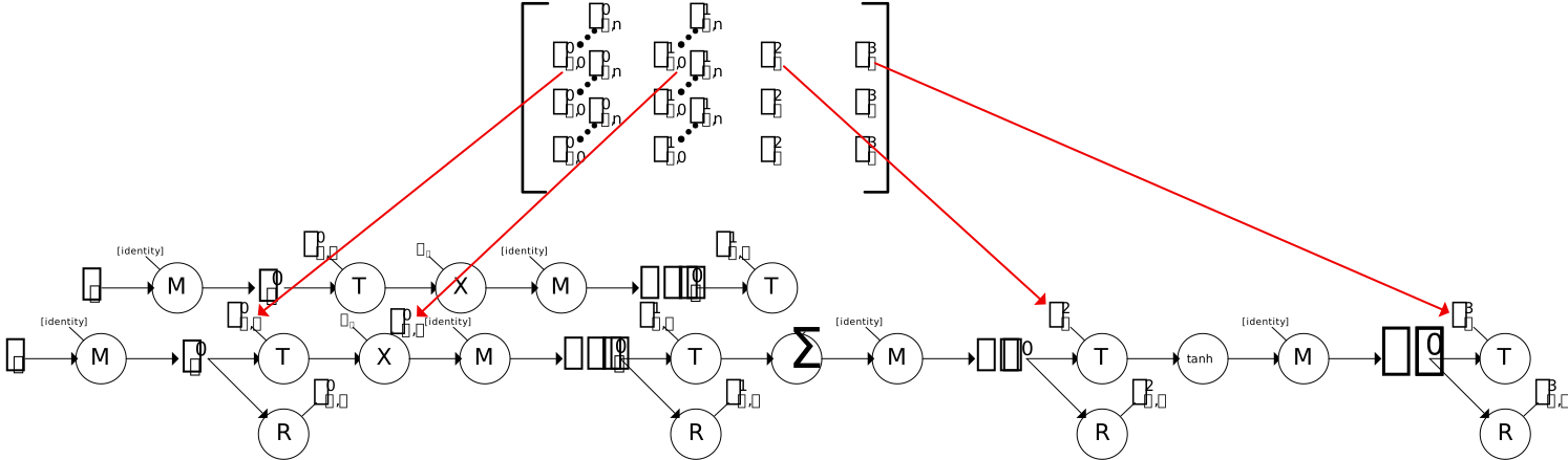
Arena organizes pointers into DAG
(2) Methodology: all tests use 10 seeds x 200 epochs x 80/20 shuffle-split per seed. Wine and breast were z-scored per-seed on the training portion. Learning rates: iris 0.05 for MLP and N2S, all others 0.005; SS uses 0.001 across the board. All N2S runs use num_reflections=1 (a two-stage Reflectron). Full per-seed data, per-dataset architecture shapes, and per-arm parameter counts are in the Data & Tables page.
(3) I can imagine using this framework to quantify the network’s behavior in these terms. For example, we could say the average information density of a signal in a layer is the sum of all possible inputs divided by number of signals, or the span of all the vectors in that layer’s feature set divided by the number of vectors. The information density gain would be the change in information density between two (possibly non-consecutive) layers. Alternatively something like “the log of the ratio between the information density of Layer B and Layer A.” I will admit this isn’t a really fleshed out model, is loosely analogous to the introduction from Shannon’s “A Mathematical Theory of Communication”, and likely has already been researched. But I find it fun to think about.
(4) See param_diff.c
(5) A small trap I ran into: under glibc, srand(0) and srand(1) produced byte-for-byte identical output sequences; the seeds 0 and 1 map to the same internal state. When some of my tests showed seed 0 and seed 1 producing identical results, I thought this was a bug in the training loop; there wasn’t. Seeds were transitioned to use 1…N for all reported runs.