Update 1: uGrad & NN in C

I recently learned about Autograd and Neural Nets. The Python implementation makes the algorithms seem simple; writing them in C showcased the amazing complexity hidden underneath.

Now I understand why everyone uses Python.

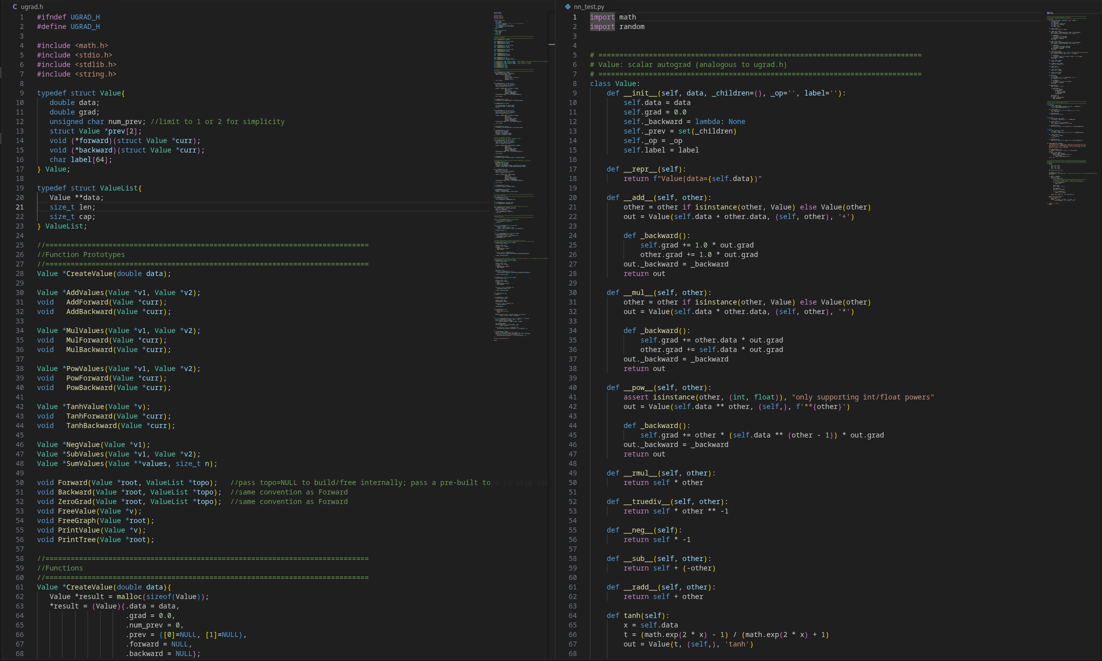
Python (with NumPy/PyTorch) lets you represent operations at a higher level of abstraction than C. At an abstract level, the algorithms are simple. We benefit from decades of study and refinement; it’s amazing how these ideas have matured and crystallized. Karpathy’s first “Zero-to-Hero” lecture drives home how basic the ideas can seem when presented at a high level. Following along in Python gave me a conceptual understanding and a feel for the algorithms.

However, I developed a habit of stubbornly persisting with C. This has fueled (and been fueled by) a belief that implementing something in C requires an intimate understanding of how data flows through your software; something you can’t quite get from Python (this also applies to my belief that pointers are the most beautiful thing in programming*). So I decided to re-implement both algorithms in C.

They are conceptually simple–but complex in scale. The devil is in the details and the implementation has a lot of details.

uGRAD.h

The Python implementation looks very clean. Declaring every variable/value in the arithmetic as an instance of a custom class and overloading the operators lets you define what connections should be made inside the Value class abstraction; from then on it happens under the hood. Adding a layer of complexity does not require expanding the architecture.

It takes more effort in C. Keeping track of all the data objects in the graph–what each instance contains, and what each instance connects to–is a challenge. Instead of a Python class that encapsulates everything, I used structures containing rigidly typed members and pointers. Including pointers to functions.

In Micrograd, instances of the Value class are nodes in a graph that connect to other Value nodes in a tree, from left to right. Nodes need to track the math operations being performed: they contain functions that describe how data passes through each node. This includes the backward propagation (for autograd). It also includes the forward propagation: how the output is determined by the inputs. The Forward operations are abstracted away so fast it’s hard to notice that it was implemented.

The Python engine can construct the Value DAG on the fly as it encounters any operation on a Value–once the class is fully defined, it can be used like a standard double.

C doesn’t afford you these luxuries. For example: the C Value struct contains the same basic variable members as micrograd’s Value class: the numerical value of the node and gradient. The data “backbone” of the autograd algorithm is a Directed Acyclic Graph, a branching structure extending from leaves to the root. I like to think of it as a tree stretching across a 2D plane from inputs to output. A node has to contain these relationships. My Value struct represents these edges using Value * pointers. Finally, the Value node requires some way to “contain” the Forward() and Backward() operations. But there are no objects, operator overrides, or function encapsulations in C. We only have the most powerful tool: pointers.

C is very straightforward about its data**. There are basic types, typed variables, and operators for those variables. Functions allow me to encapsulate and re-use a set of operations, but all these tools are somewhat inflexible. Pointers grant you infinite flexibility. Pointers allow you to indirectly access data in memory from anywhere in your program, like stars in the sky: visible from anywhere in the world**.

One powerful feature of pointers is that they can point to any data, not just variables allocated in the heap. Including functions. My Value structs “encapsulate” various operations by containing as members pointers to functions implementing those operations.

What operations are necessary?

• Forward computation (inputs to output)
• Backward computation (output back to gradient)
• An implementor function

The first two are referenced inside each Value using pointers; for example AddForward() and AddBackward(). The implementor function is analogous to the Python’s init constructor: it connects the two operand Values into a single root. This requires dereferencing two pointers to Value structs, allocating a new Value on the heap, connecting the Value to the upstream nodes and to the Forward and Backward functions. Additionally, in C we need to explicitly track whether there are one or two upstream branches (Unary vs. Binary operators). This is what grows the tree. It also means that the math operations have to be explicitly implemented by calling these “constructor” functions.

I have to call myself out here: I’m using individual mallocs for each Value node, and linking them up after the fact using pointers. Traversing the value graph means randomly jumping around the heap–which might not matter for a tiny example model, but does matter for larger models or specialized hardware. Allocating an arena (a chunk of memory) and then dispensing Value-sized units of that chunk would be more efficient.

The Value struct has to encapsulate the Forward and Backward functions because they need to be invoked programmatically. Autograd works by iterating through all the nodes, from the root to the leaves, calling a unique Backward() function for each. Likewise, computing the mathematical expression the tree represents requires calling a custom Forward() function on each node from the leaves to the root. Python’s abstraction mechanisms handles all this for you.

In C, functions pointed at by a struct member must have identical parameter lists. I can’t mix AddForward(Value *a, Value *b) and PushForward(Value *a). In order to accommodate the existence of both binary and unary operations, all this information has to be encoded into members of the Value struct, and the Value struct itself is passed into each Forward() and Backward() function, where the information can be decoded.

Which means iterating through each node requires you to:

1. Read the Value struct pointer to function pointer member
2. Call the pointed at function, passing the Value struct address into it
3. From within the pointed at function, read the Value struct pointer array to the address of each upstream Value node

I used pointers a lot.

I believe any Python/C++ implementation is going to work similarly under the hood; however, a significant architectural difference emerged between the two implementations as a result of the language differences.

My version constructs the DAG explicitly by calling functions representing each math operation. The graph is constructed once and then retained in memory for future use. This is why I need the additional Forward() function to propagate new inputs into the expression; Python constructs the graph on-the-fly whenever the interpreter needs to process some expression, which makes it easier to modify/experiment.

This also means I have a lot more setup/tracking to do when I want to expand/modify the graph, which will come into play when I use the ugrad.h implementation to make neural nets.

Neurons and an MLP

Micrograd uses a tree of Value nodes to represent an algebraic operation, like a*b+c. At its core, a Neuron is just a linear combination of features (inputs) passed through a non-linear filter (which is what sets it apart from a multivariate linear polynomial regression).

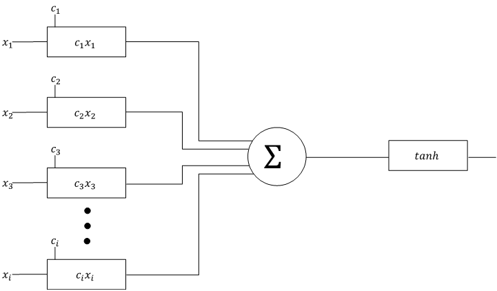
Which means implementing Neurons using Micrograd Value nodes is relatively straightforward: building a neuron means building the requisite tree of Values. Practically, I ran into the same architectural considerations as before. A Neuron has to store:

• Weights
• Features
• Products (intermediary)
• Output

The features have to be stored even though they aren’t part of the backpropagation because I can’t mix and match types in C like you can in Python (or in C++ with something like templates). It was cleaner to elevate the input values from a double to a full Value than it would have been to use unions, or implement separate functions and logic to handle leaf nodes. This keeps the graph logic clean: the first feature (index 0) is initialized with a dummy value of 1.0, which effectively makes the first weight a learnable bias. This way every neuron gets a bias without any special-case code or additional members in a struct.

The number of weights, features, and products are all dynamically allocated structs, so I implemented them as a double pointer. This lets each member be a 2-dimensional structure allocated at runtime. Each row can be a different length as well! This served as the first example of what I consider to be the “vertical interconnections” of the algorithm. The Value graph exists in a single plane; the Neuron itself only contains references to nodes in that graph; hooks from this abstract idea of a “Neuron” down into the actual implementation of the underlying math.

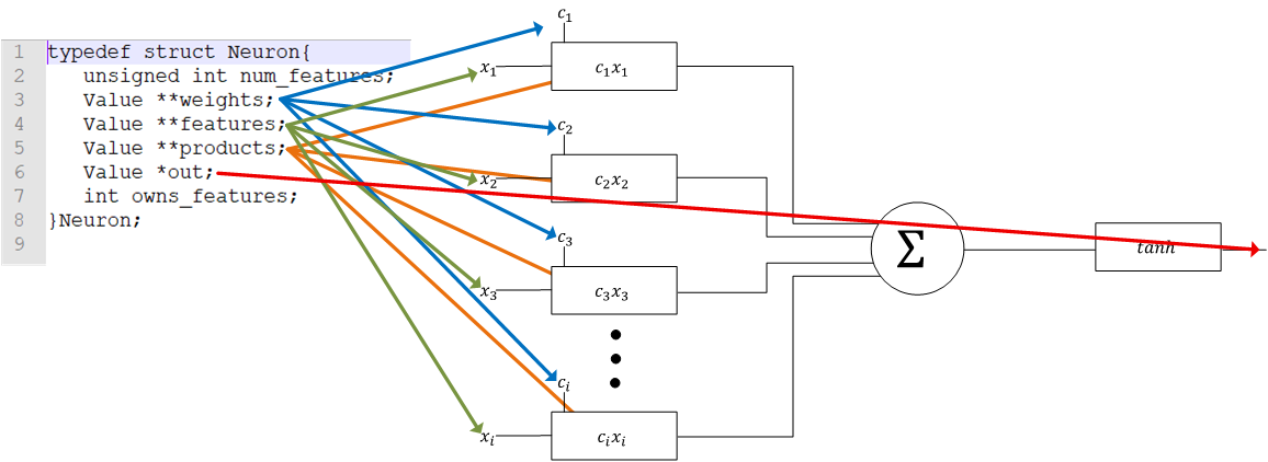
The function that creates the Neuron generates the graph, allocating nodes on the heap and connecting them to each other using pointers. Pointers in the Neuron reach down into the Value graph, hooking into individual nodes. Implementing the Layers and the MLP data structure is similar: they are structs that create multiple neurons/layers, connect them together using pointers, and hook each down to the next lower level of abstraction (Neurons get hooked into Layer instances, Layers into the MLP instance).

All you really need is the output Value node; everything else is for conceptual organization. To reach any particular node in the graph you can either: (1) walk backward from the output node, or (2) chain indirection operators from the most abstract struct downwards. Copying these pointers to a top level array in the MLP struct is more convenient when trying to connect layers together or otherwise iterate through the output Values of the various units in the design.

This is one area in which I could improve the memory allocation scheme. Instead of scattered mallocs to the heap, I could allocate an arena for each Neuron. This memory region would then contain all the encapsulated values (features, weights, intermediary values) in contiguous memory. This scheme could be extended up the layers of abstraction: from Neurons to Layers (collections of Neurons) and from Layers to MLP (a collection of Layers).

The Tree-Of-Trees, or Yggdrasil^2

The result of this is a kind of “Tree-of-Trees”. Each layer of abstraction is its own tree: the Value DAG, the Neuron Network, the Layers, and finally the single-node MLP “tree”. All of these are connected together vertically into another orthogonal tree: the root being the most abstract concept (the MLP) down to the most concrete: the Value nodes.

For example: consider a 2-input, 1-output MLP with a single, 2-Neuron intermediary layer. The DAG of Value nodes contains ~20 nodes between all the weights, features, products, etc.. All these nodes are connected laterally through mathematical operations. Above it is the Neuron level. There are three Neurons: two in the hidden layer, one output. Each of these Neurons hooks down into corresponding Value nodes in the DAG below. The Layer level has two nodes, one for the hidden layer and one for the output, each hooking down into their respective Neurons. Finally, the MLP level is a single node pointing down to the Layers.

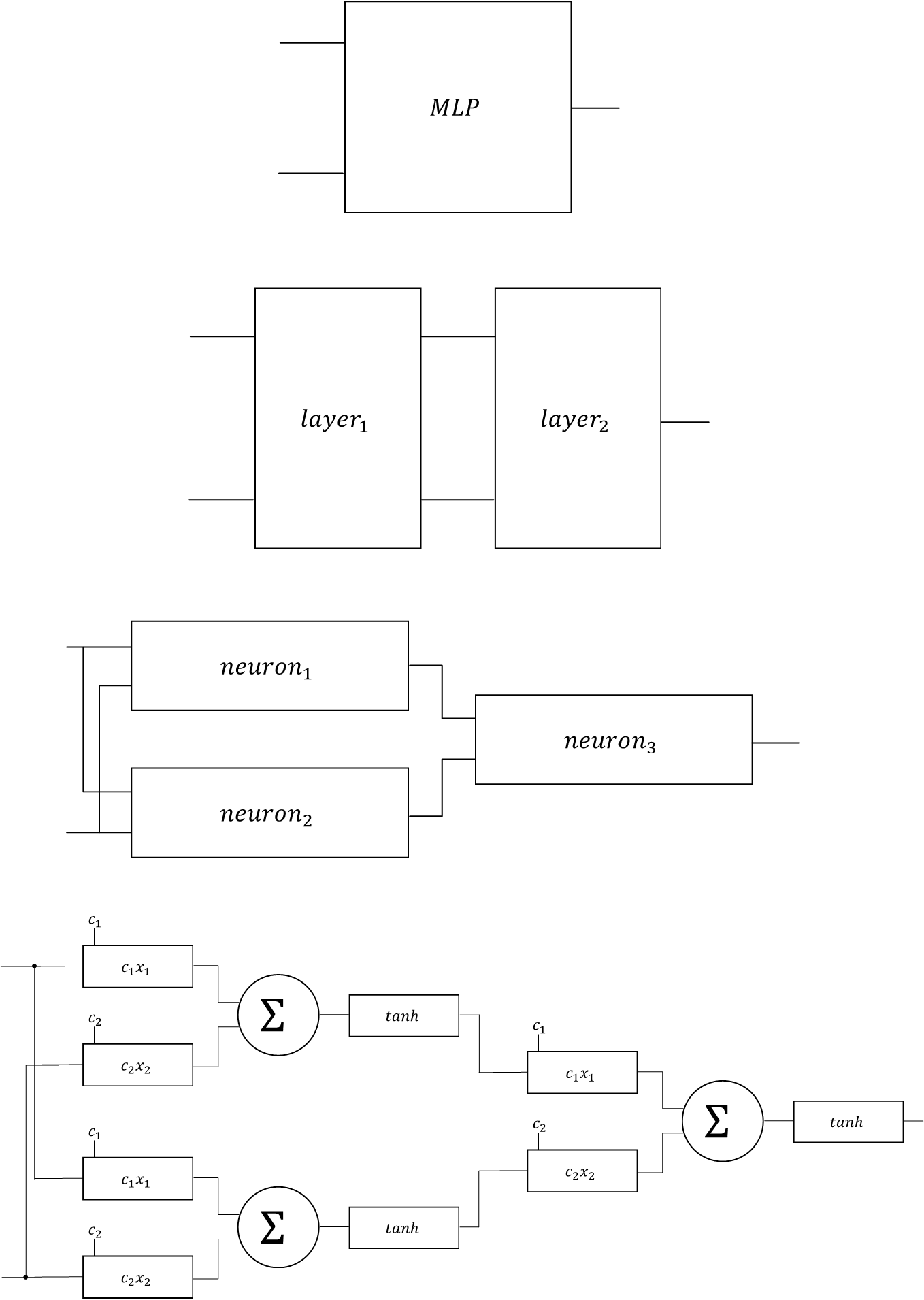
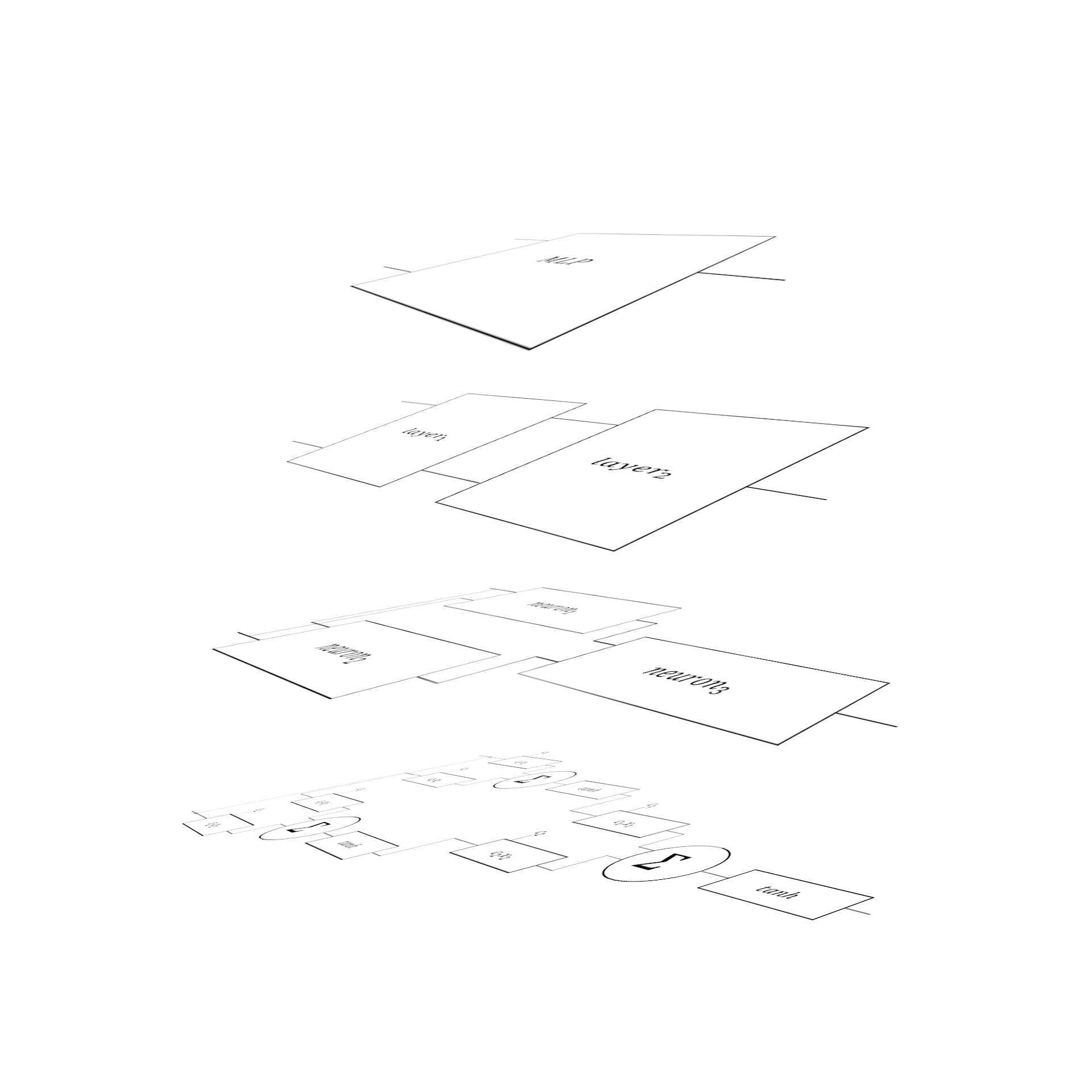
The horizontal trees (DAG, Neural Network, MLP) represent computation–the flow and mixing of signals as they permeate through the system, flowing from input to output and back, in the case of backpropagation while training. Horizontal edges represent arithmetic. The vertical tree represents abstraction: it is the architecture of MLP algorithm, the organization of individual units into conceptual wholes. The vertical tree’s edges represent concretizing in implementation the abstract concepts.

Free() strategy

C makes painfully clear how intertwined every piece of data is. There are lateral connections through the Value graph and vertical connections through different “layers” of the program: a Value can simultaneously be a node in the Value Graph, the output of a neuron, and the output of a Layer in the MLP. Both algorithms–the autograd algorithm used for backpropagation and the MLP algorithm used for interpolation/extrapolation–use this data. Moreover, the features and weights are symmetric in my implementation: both are Value pointers contained within the Neuron. Functionally they are antisymmetric: autograd is used to modify the weights; usage of the MLP changes the features. Both are modified while training the model. Looking at it feels like looking at the fibers of leather, or velcro: two sets of threads intertwined and tangled together to form an inseparable whole.

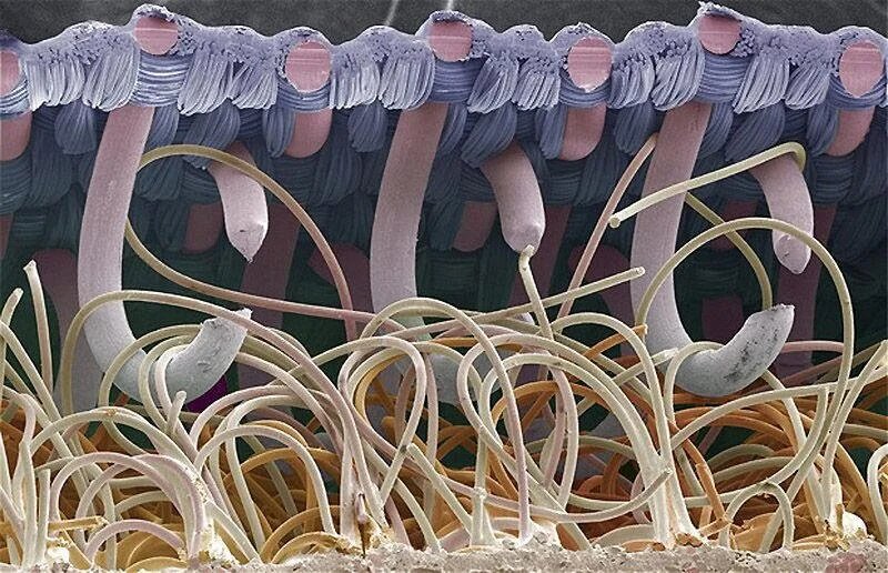
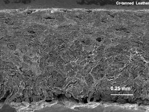
Which makes deallocating all this data kind of a pain. At least when compared to Python. Python hides the physical reality that all this data has to be placed somewhere in memory, ideally using a thought-out strategy–and has to be removed from that memory when the program terminates.

I avoid double-frees while untangling this knot of pointers by implementing explicit ownership tracking with an “owns_features” flag in each Neuron struct. When a neuron’s features are actual outputs from a previous layer, the pointers belong to a different branch of the verticle tree, and the current neuron must not free them. Without this flag two neurons would both try to free the same Value nodes.

Data needs to be freed from the top, down. The MLP frees the Layers before freeing the pointer to the layers’ pointer array and then itself; Layers does the same with its neurons (and then itself); and each neuron frees each constituent value node starting from the output and moving backwards to the weights and features. The data is linked together in a tree of pointers that represents the vertical organization of the MLP, where each layer represents a more abstract representation of the underlying data.

Deallocating the MLP means walking the vertical tree from root to leaves–from MLP down to the Value nodes. The pointers in each layer flow downwards, and the free algorithm has to follow that flow. The vertical tree dictates the order of destruction in the same way that the horizontal tree dictates the order of computation.

Note: Training & Convenience

An additional architectural decision is the addition of a Trainer struct. The autograd algorithm needs a final Value to serve as the root of the tree; since I permit the MLP to have multiple outputs I use the final loss function as root. The trainer encapsulates the target values and caches the topology list used by the Backward() and Forward() algorithms. This required modifying the uGRAD functions to optionally accept a pre-computed topology. Deallocation also has to start from the Trainer struct: Values that are not part of the MLP topo graph, the target values, the topo value list’s data, and finally the topo value list pointer itself.

The Autograd works by taking the graph of Value nodes and sorting them from root to leaves, in order to iteratively compute the partial gradient of each node based on how a small change in the node affects the next root-ward node in the tree, starting from the root. At the end, this gives you how changing each input affects the output value. In Python, the graph is computed every time Backward executes, so the topology also has to be re-computed each call. Since my implementation assumes the graph is always valid, I can compute this topology after the graph is set up and cache it to save time.

Storing the topology graph opens up an opportunity for optimizing memory use: walking through the topology is the most frequent traversal: walking forward to use the model, backwards to train it. Moving all the nodes in the Value graph from random (or randomly chunked) locations in the heap to a single arena, arranged in the order of the DFS micrograd uses, would place them in consecutive memory locations. This would make iterating through the topology a sequential scan through memory***.

All this aligns with the overarching theme of translating to C: the structure of the data is somewhat rigid: explicitly constructed and then re-used throughout the program. The knot of malloc’ed pointers also require explicit clean-up. The Trainer struct itself isn’t really a deviation from the Python version; the Lecture had the functionality but I wrapped it into a struct for convenience.

Final thoughts

I rarely work with data that is as intertwined as what I’ve seen here: layers of data structures with pointers hooking each into the others. Writing code that implements all these hooks by hand forces you to appreciate the scale of the graph under the hood–both in the number of nodes and interconnections. Even for an extremely small MLP.

The data is not just highly interconnected. The edges of the graph represent different relationships between data nodes. Some edges represent propagation of the input signals forward from inputs to output, others represent the gradient. Some edges represent the connections between neurons. Other edges move up and down the abstraction tree–taking nodes from the ground floor (the tree of mathematical operations used to compute the MLP output and autograd) and connecting them to a member of the Layer or MLP struct instance. The functions themselves are accessed via pointers–which means some edges represent branches in code execution! It is this complexity–that doesn’t just span the basic “2D” plane of a traditional algorithm’s data flows, but extends into a kind of third dimension that represents “abstraction” which possibly gives rise to the wonderfully emergent features we find useful.

You can find the code here: ugrad.h & nn.h

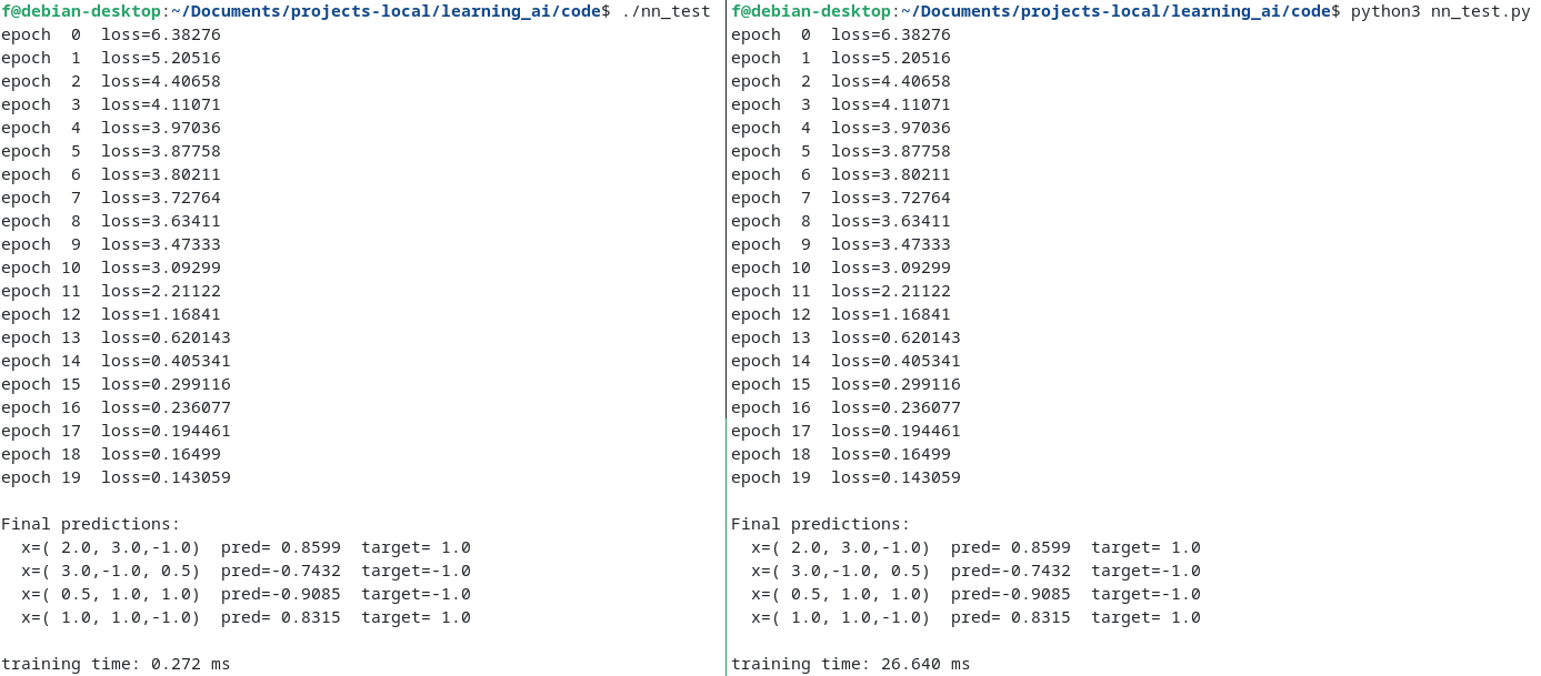
*I love pointers. **Some might say dumb, I prefer honest. ***This leads down a rabbit hole of van Emde Boas layouts and structure-of-arrays vs. array-of structures, but I digress.